Warning message:
“package ‘DropletUtils’ was built under R version 4.4.3”
Warning message:
“package ‘SeuratObject’ was built under R version 4.4.3”
Show code
# # another options for vscode for plotting# options(repr.plot.width = 10, repr.plot.height = 5, jupyter.plot_scale = 1)# # make the resolution betteroptions(repr.plot.res =300) # set dpy to 200
main_folder <-"/home/kharuk/projects/courses/st_daad/data"# Change to your actual path# List all sample directories inside the main foldersample_dirs <-list.dirs(main_folder, recursive =FALSE)print(sample_dirs) # Check detected directories
Show code
sample_id <-"GSM6171784_PSAPP_CO1"
Show code
# upload one sample for preprocessingspe <-read10xVisium(samples = sample_dirs[1],sample_id ="GSM6171784_PSAPP_CO1",data ="filtered",type ="sparse",images ="lowres",load =TRUE)
Show code
# move rownames to rowData names new column ensembl_idrowData(spe)$ensembl_id <-rownames(rowData(spe))
Sample preprocessing
Plot data
Show code
# plot spatial coordinates (spots)plotSpots(spe)
QC metrics
Show code
# First, we subset the object to keep only spots over tissue.# subset the object to keep only spots over tissuespe <- spe[, colData(spe)$in_tissue ==1]dim(spe)
# calculate per-spot QC metrics and store in coldata spe <-addPerCellQC(spe, subsets =list(mito = is_mito))head(colData(spe))
Selecting thresholds for filtering
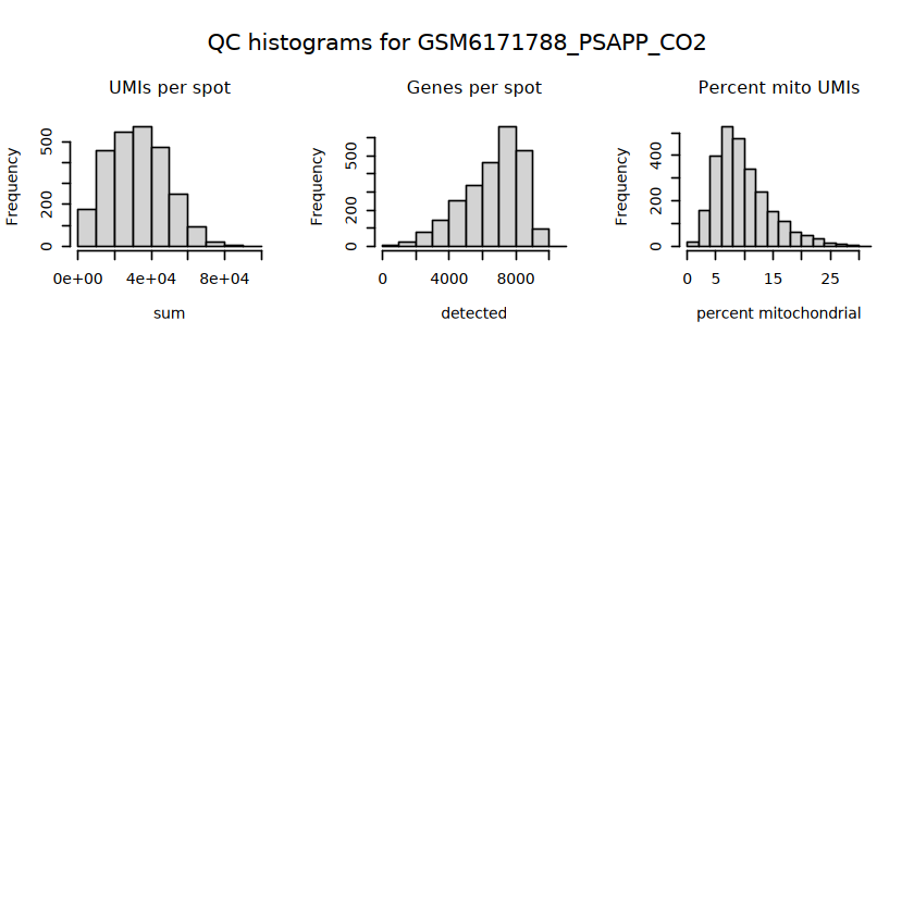
Have to select thresholds for several QC metrics: (i) library size, (ii) number of expressed genes, (iii) proportion of mitochondrial reads, and (iv) number of cells per spot (does not exist in data).
Library size represents the total sum of UMI counts per spot.
Show code
hist(colData(spe)$sum, breaks =20)
Show code
colData(spe)
Show code
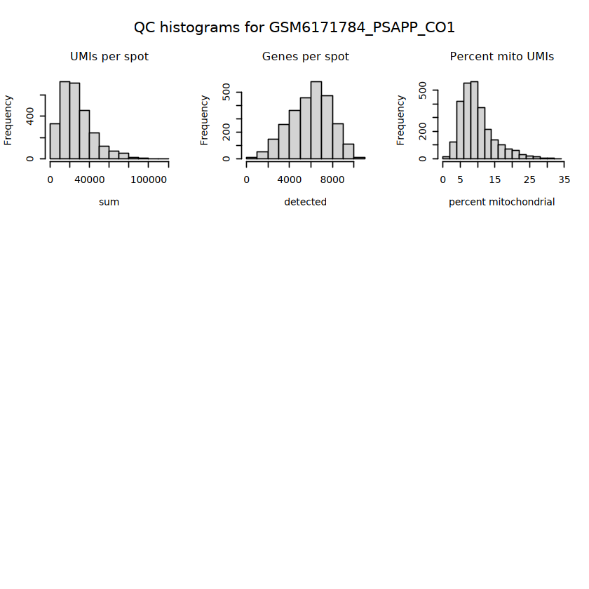
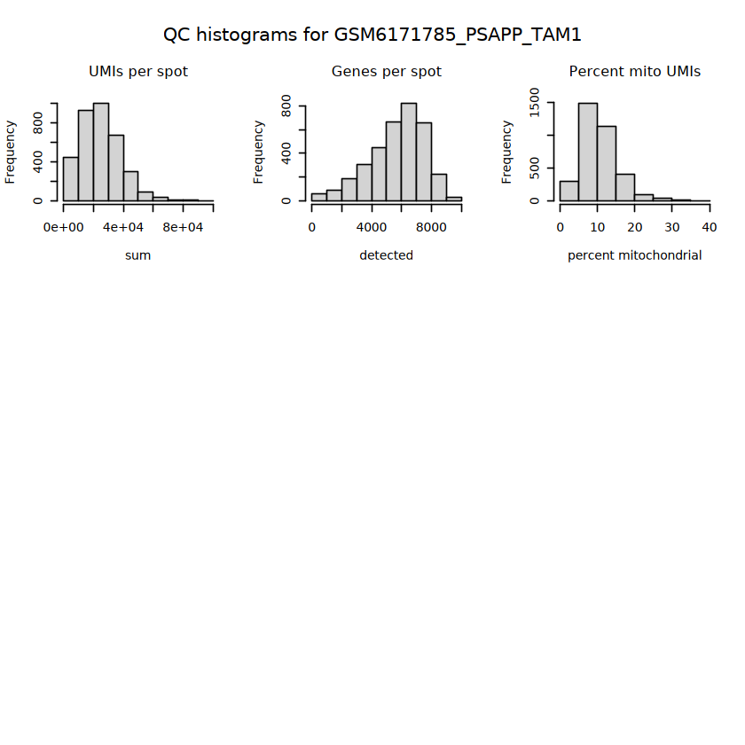
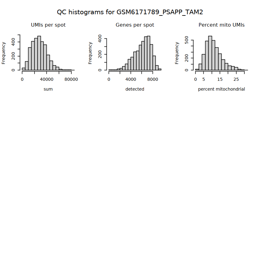
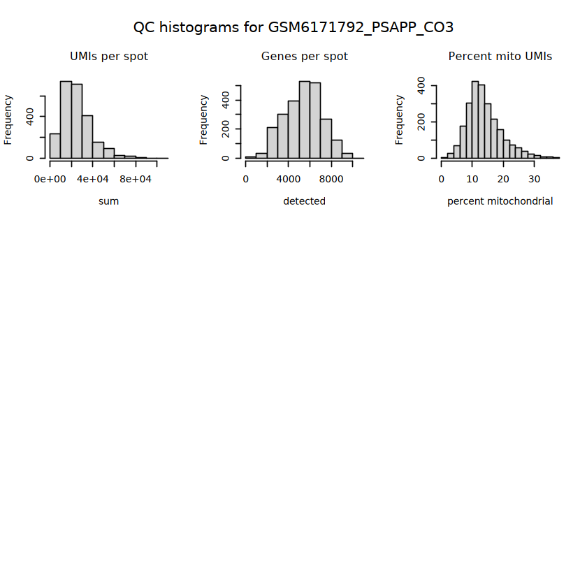
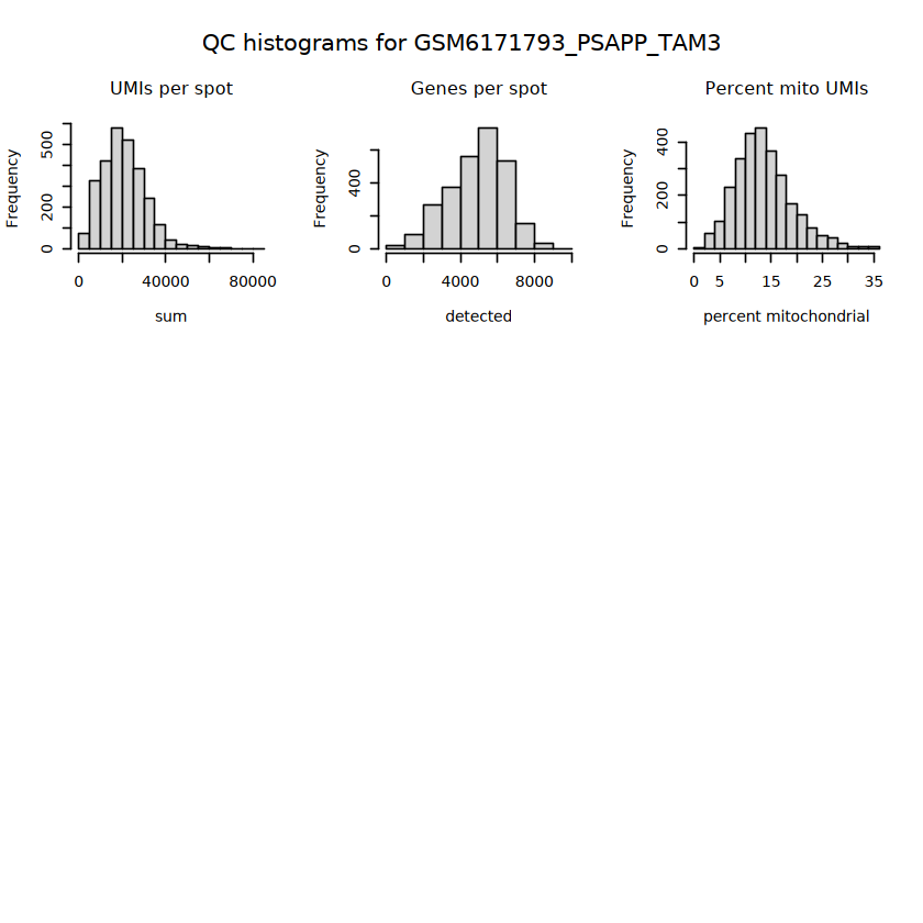
# histograms of QC metrics before filteringpar(mfrow =c(3, 3))hist(colData(spe)$sum, xlab ="sum", main ="UMIs per spot")hist(colData(spe)$detected, xlab ="detected", main ="Genes per spot")hist(colData(spe)$subsets_mito_percent, xlab ="percent mitochondrial", main ="Percent mito UMIs")# hist(colData(spe)$cell_count, xlab = "number of cells", main = "No. cells per spot")
Show code
# asign gene names for plotting rownames(spe) <-rowData(spe)$symbolcolData(spe)$sum <-colSums(counts(spe))
Show code
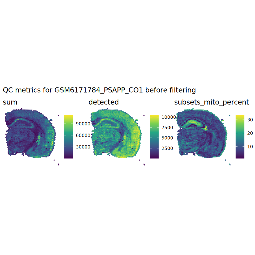
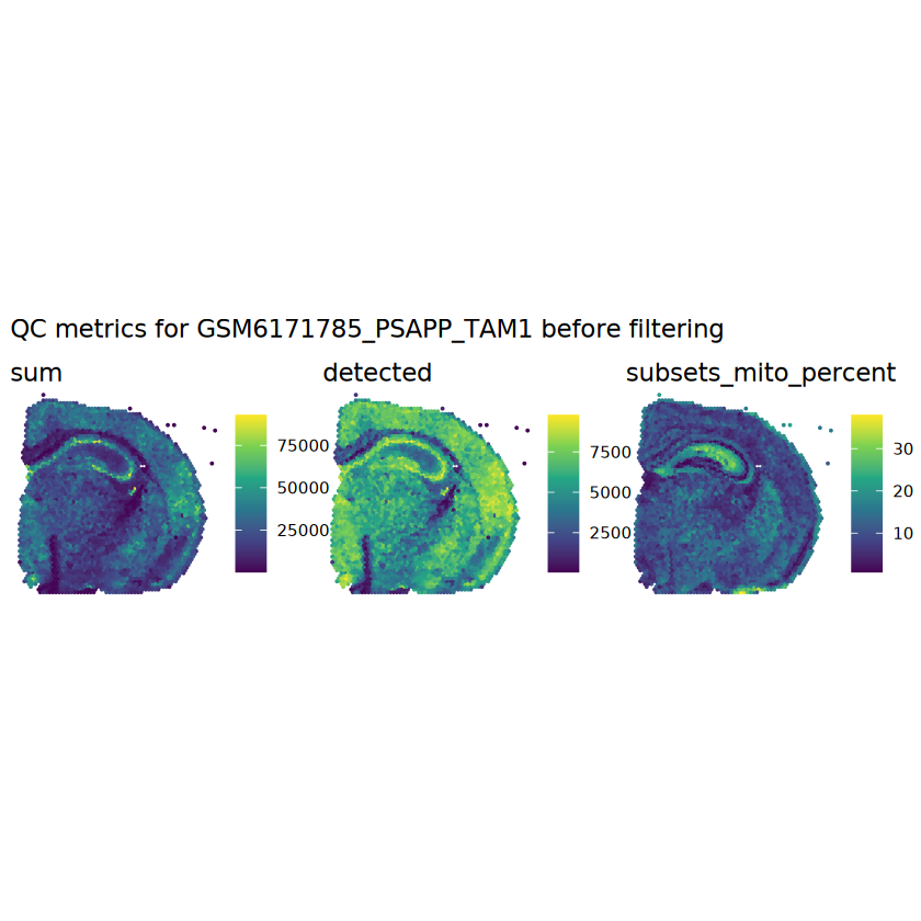
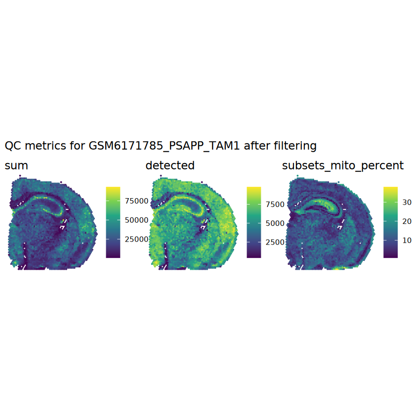
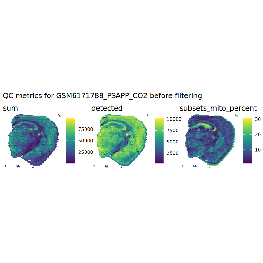
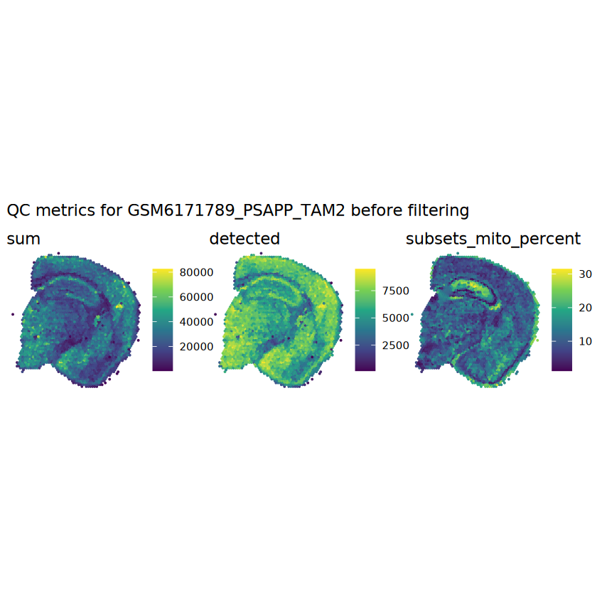
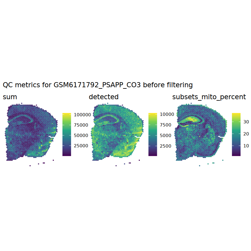
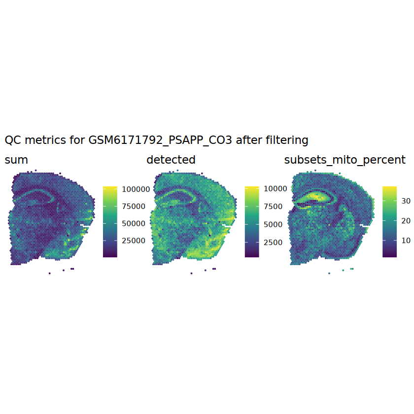
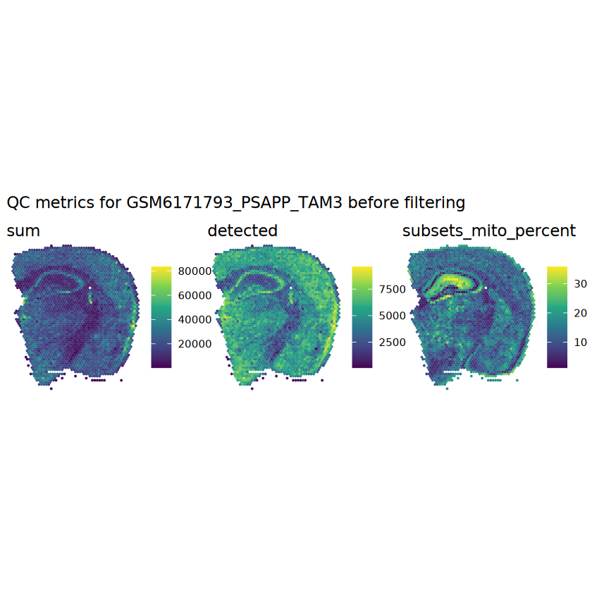
# plot the same QC on the spatial coordinatespal <-c("#fde725", "navy")p1 <-plotSpots(spe, annotate ="sum", pal ="viridis", point_size =0.03) +theme_void()p2 <-plotSpots(spe, annotate ="detected", pal ="viridis", point_size =0.03) +theme_void()p3 <-plotSpots(spe, annotate ="subsets_mito_percent", pal ="viridis", point_size =0.03) +theme_void()aqc_before <-wrap_plots(p1, p2, p3, nrow =1) +plot_annotation(title =glue("QC metrics for {sample_id} before filtering"))qc_beforeggsave(filename =glue("qc_metrics_{sample_id}_before_filtering.png"), plot = qc_before, width =10, dpi =300)
Another option is to calculate MAD and filter based on this value.
Show code
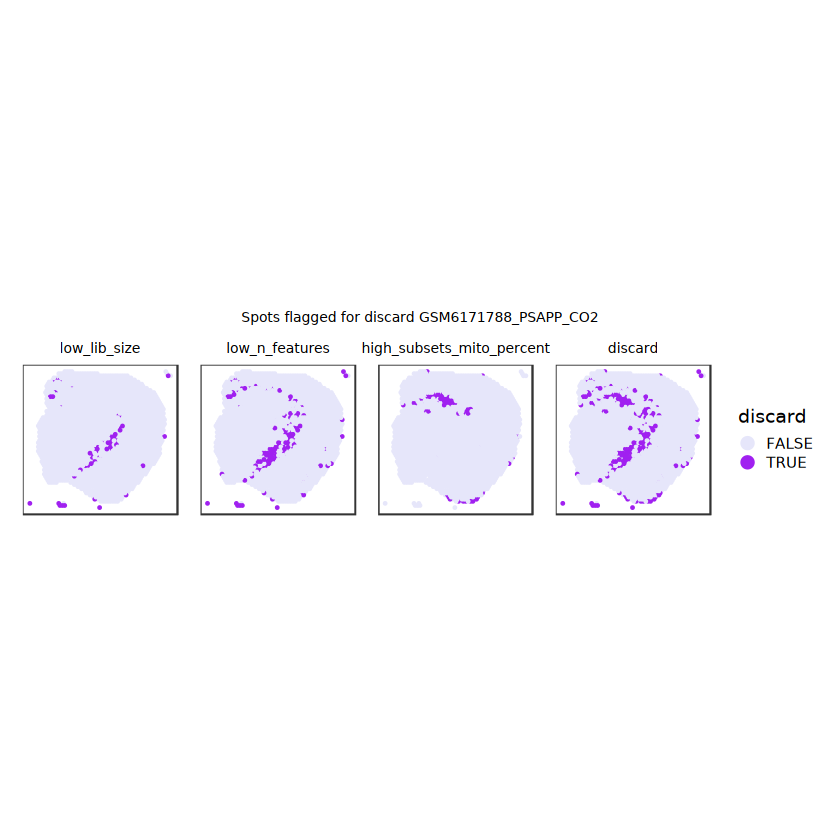
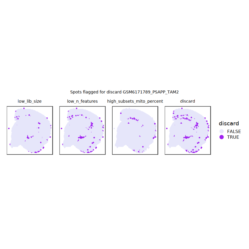
# determine outliers via thresholding on MAD from the medianol <-perCellQCFilters(spe, sub.fields="subsets_mito_percent")# add results as cell metadatacolData(spe)[names(ol)] <- ol # tabulate # and % of cells that'd # be discarded for different reasonsdata.frame(check.names=FALSE,`#`=apply(ol, 2, sum), `%`=round(100*apply(ol, 2, mean), 2))
Show code
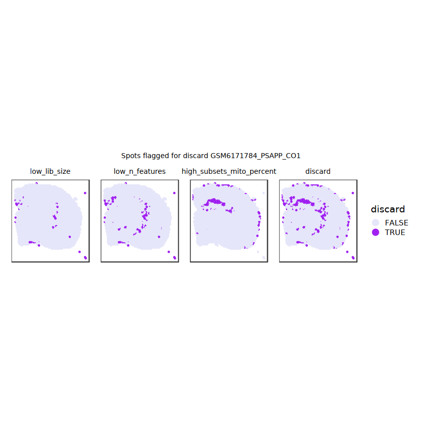
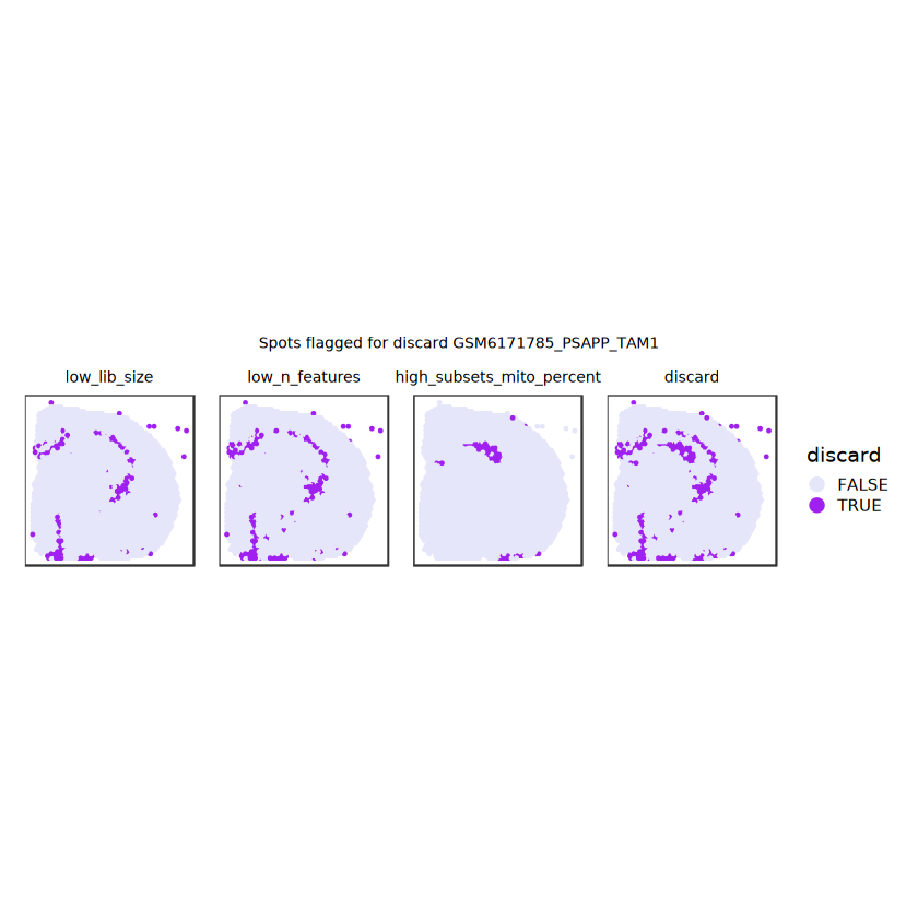
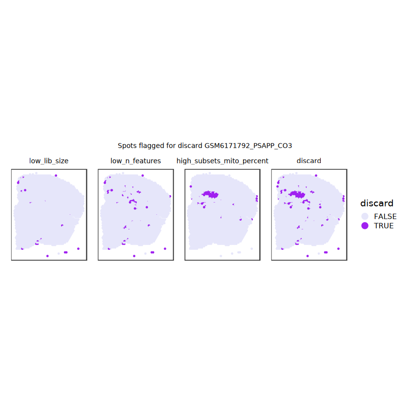
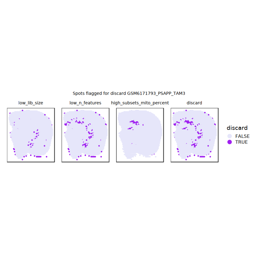
# plot what spots will be discarded with MADlapply(names(ol), \(.) plotSpots(spe, annotate=.) +ggtitle(.)) |>wrap_plots(nrow=1, guides="collect") +plot_annotation(title =glue("Spots flagged for discard {sample_id}")) &guides(col=guide_legend(override.aes=list(size=3))) &scale_color_manual("discard", values=c("lavender", "purple")) &theme(plot.title=element_text(hjust=0.5, size=8), legend.key.size=unit(0.8, "lines") )
I’d like not to remove the outliers with MAD, but to set a threshold for each of the QC metrics: library size (sum), number of expressed genes (detected), proportion of mitochondrial reads (subset_mito_percent)
Show code
# Set the threshold manually # select QC thresholdsqc_lib_size <-colData(spe)$sum <600qc_detected <-colData(spe)$detected <400# qc_mito <- colData(spe)$subsets_mito_percent > 30# number of discarded spots for each metricapply(cbind(qc_lib_size, qc_detected), 2, sum)
Show code
# combined set of discarded spotsdiscard <- qc_lib_size | qc_detectedtable(discard)
Show code
# store in objectcolData(spe)$discard <- discard
Plot the set of discarded spots in the spatial x-y coordinates, to confirm that the spatial distribution of the discarded spots does not correspond to any biologically meaningful regions, which would indicate that we are removing biologically informative spots.
Show code
plotSpotQC(spe, plot_type ="spot", annotate ="discard") +plot_annotation(title ="Spots to be discarded")
# # filter low-expressed and mitochondrial genes# # using very stringent filtering parameters for faster runtime in this example# # note: for a full analysis, use alternative filtering parameters (e.g. defaults)# # re-calculate logcounts after filtering# # using library size factorsspe_nnSVG <-logNormCounts(spe)# # # run nnSVG# # using a single core for compatibility on build system# # note: for a full analysis, use multiple coresset.seed(123)spe_nnSVG <-nnSVG(spe_nnSVG, n_threads =6)# # # investigate results# # # show resultshead(rowData(spe_nnSVG), 3)# # # number of significant SVGstable(rowData(spe_nnSVG)$padj <=0.05)# # # show results for top n SVGsrowData(spe_nnSVG)[order(rowData(spe_nnSVG)$rank)[1:6], ]# # # identify top-ranked SVGrowData(spe_nnSVG)$symbol[which(rowData(spe_nnSVG)$rank ==1)]
Preprocess all samples
Show code
# upload samplesmain_folder <-"/home/kharuk/projects/courses/st_daad/data"# Change to your actual path# List all sample directories inside the main foldersample_dirs <-list.dirs(main_folder, recursive =FALSE)print(sample_dirs) # Check detected directories
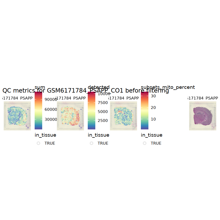
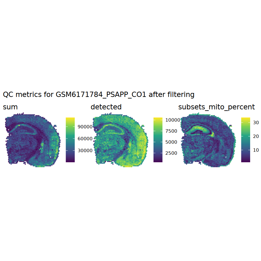
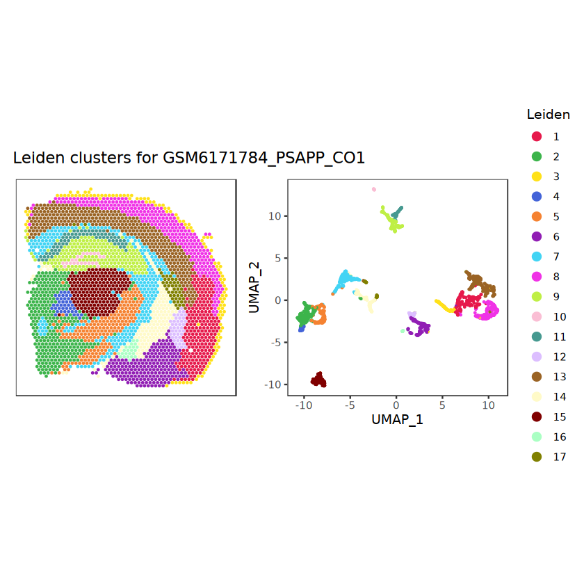
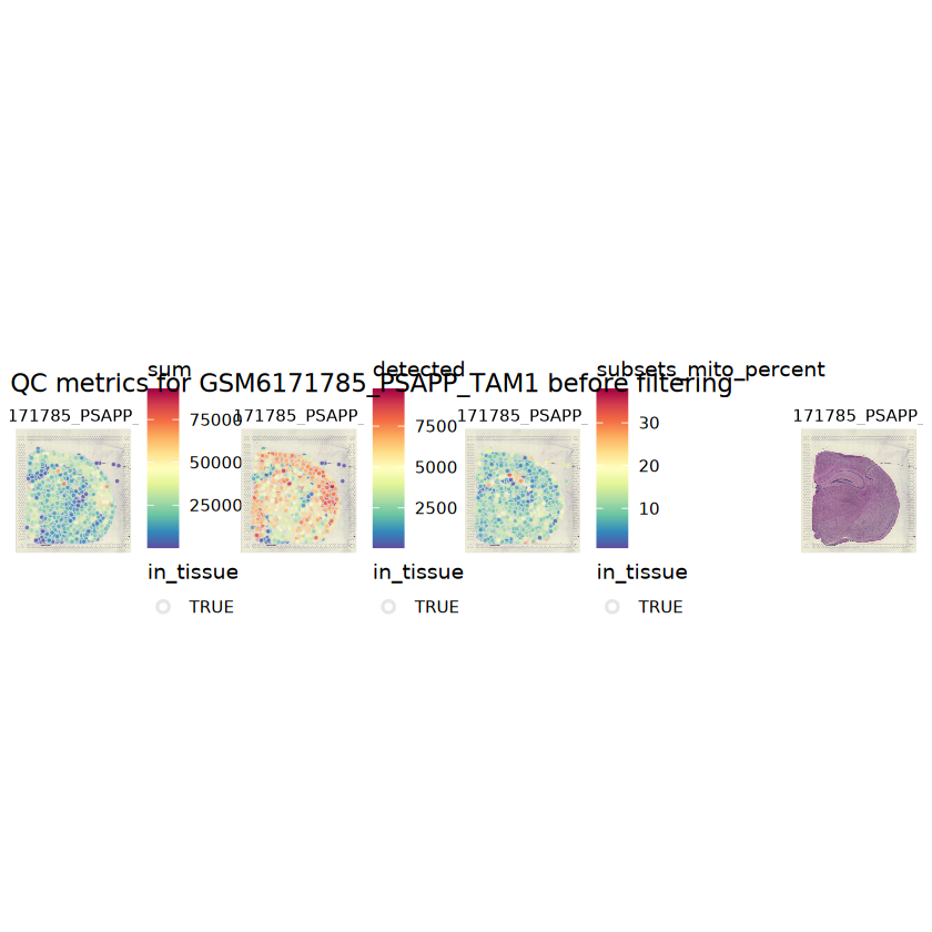
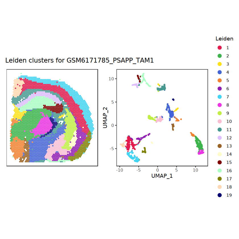
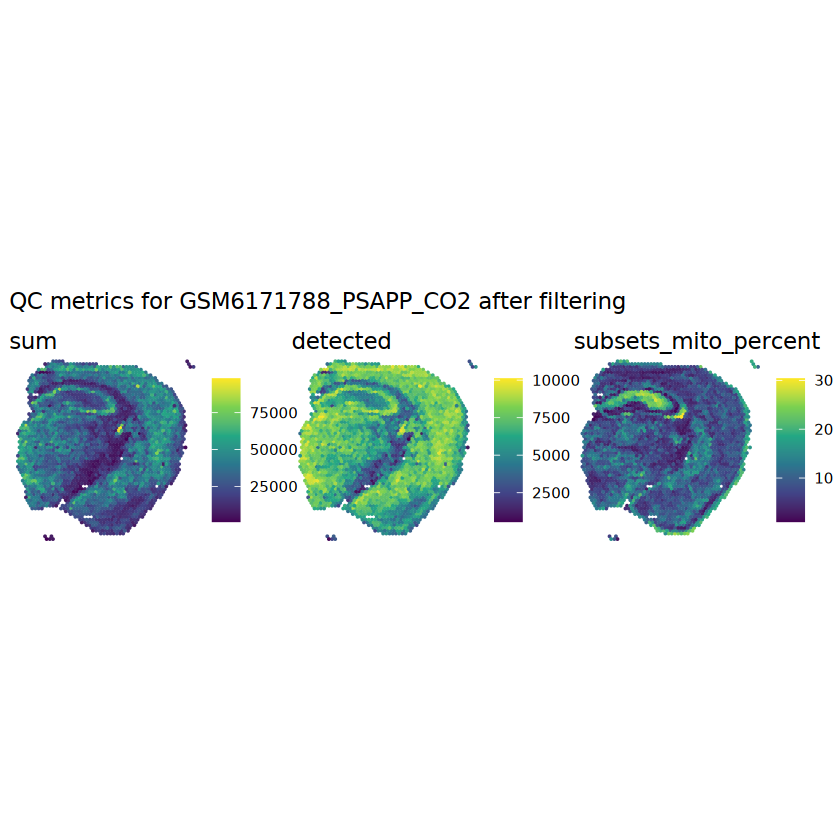
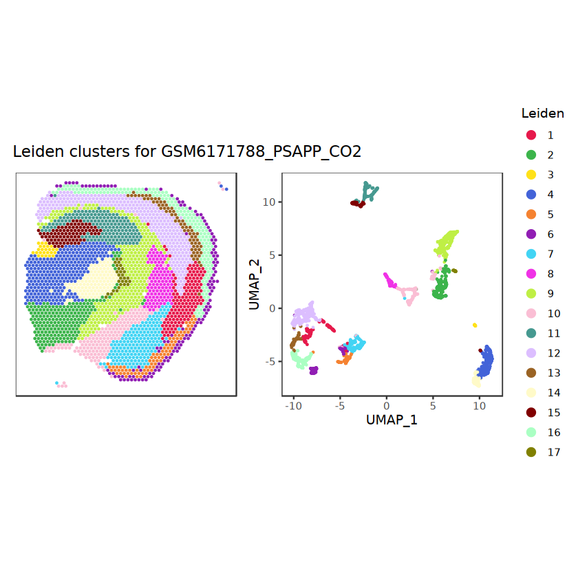
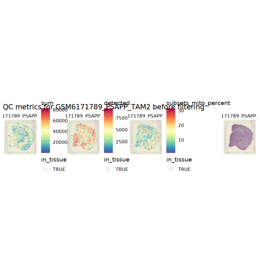
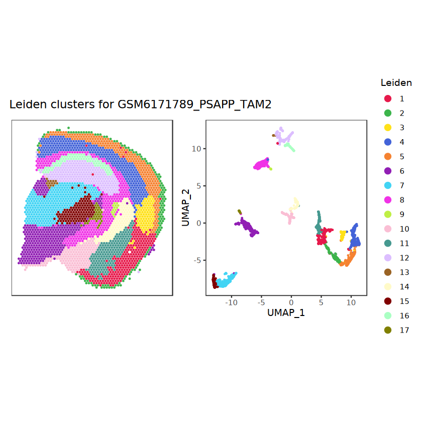
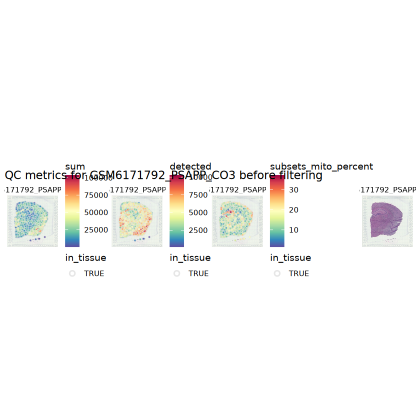
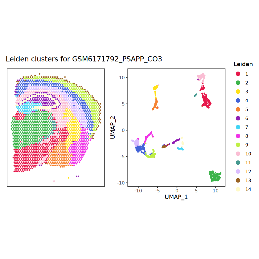
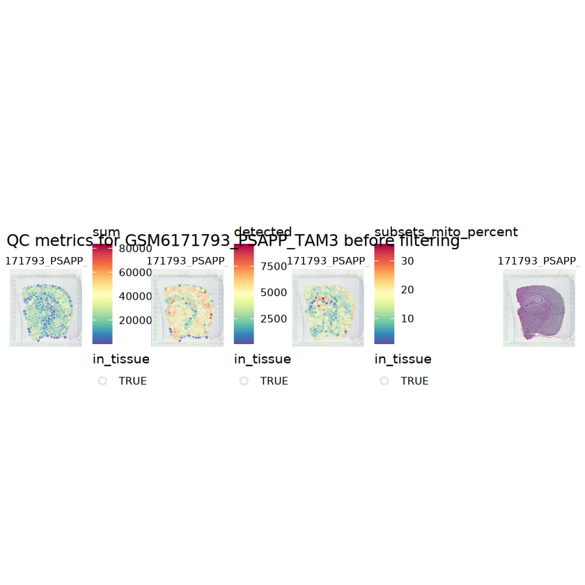
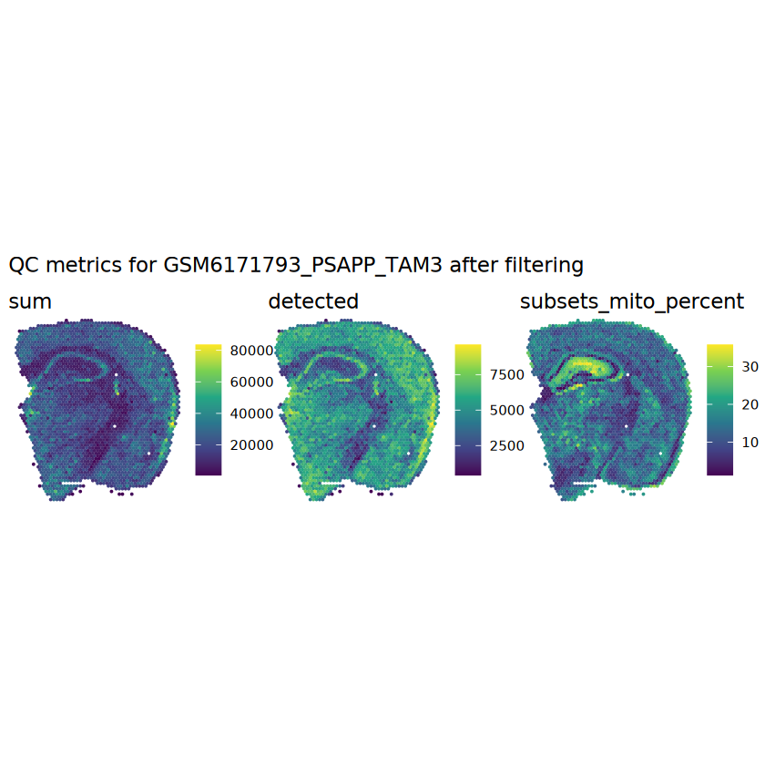
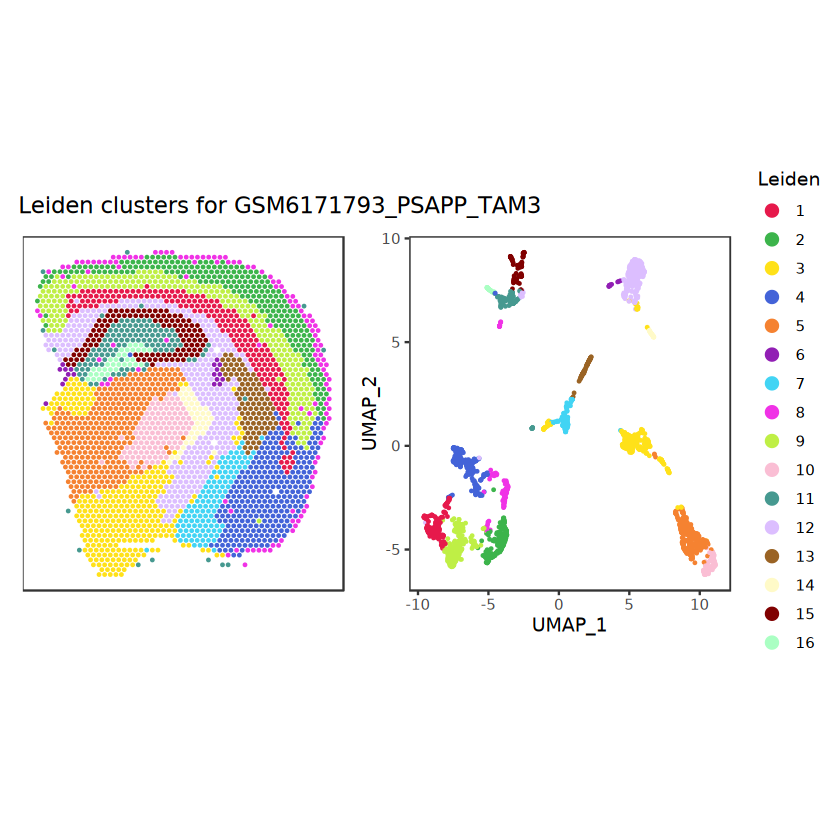
# function to preprocess a single samplepreprocess_sample <-function(sample_path) { sample_id <-basename(sample_path) spe <-read10xVisium(samples = sample_path,sample_id = sample_id,data ="filtered",type ="sparse",images ="lowres",load =TRUE )# First, we subset the object to keep only spots over tissue.# subset the object to keep only spots over tissue spe <- spe[, colData(spe)$in_tissue ==1]dim(spe)# identify mito genes is_mito <-grepl("(^MT-|^mt-)", rowData(spe)$symbol)table(is_mito)# calculate per-spot QC metrics and store in coldata spe <-addPerCellQC(spe, subsets =list(mito = is_mito))head(colData(spe))# histograms of QC metrics before filtering # TODO add title here png(glue("qc_hist_{sample_id}.png"), width =1000, height =800)par(mfrow =c(3, 3), oma =c(0, 0, 3, 0)) # layouthist(colData(spe)$sum, xlab ="sum", main ="UMIs per spot")hist(colData(spe)$detected, xlab ="detected", main ="Genes per spot")hist(colData(spe)$subsets_mito_percent, xlab ="percent mitochondrial", main ="Percent mito UMIs")mtext(glue("QC histograms for {sample_id}"), outer =TRUE, cex =1)dev.off()# asign gene names for plotting rownames(spe) <-rowData(spe)$symbolcolData(spe)$sum <-colSums(counts(spe))# plot the same QC on the spatial coordinates pal <-c("#fde725", "navy") p1 <-plotSpots(spe, annotate ="sum", pal ="viridis", point_size =0.03) +theme_void() p2 <-plotSpots(spe, annotate ="detected", pal ="viridis", point_size =0.03) +theme_void() p3 <-plotSpots(spe, annotate ="subsets_mito_percent", pal ="viridis", point_size =0.03) +theme_void() qc_before <-wrap_plots(p1, p2, p3, nrow =1) +plot_annotation(title =glue("QC metrics for {sample_id} before filtering"))print(qc_before)ggsave(filename =glue("qc_metrics_{sample_id}_before_filtering.png"), plot = qc_before, width =10, dpi =300)# plot QC with image included p1 <-plotVisium(spe, annotate ="sum", highlight ="in_tissue", point_size =0.75) +theme_void() p2 <-plotVisium(spe, annotate ="detected", highlight ="in_tissue", point_size =0.75) +theme_void() p3 <-plotVisium(spe, annotate ="subsets_mito_percent", highlight ="in_tissue", point_size =0.75) +theme_void() tissue_plot <-plotVisium(spe, highlight ="in_tissue", spots =FALSE) +theme_void()# display panels using patchwork qc_tissue_plot <-wrap_plots(p1, p2, p3, tissue_plot, nrow =1) +plot_annotation(title =glue("QC metrics for {sample_id} before filtering"))print(qc_tissue_plot)ggsave(glue("qc_metrics_{sample_id}_tissue.png"), qc_tissue_plot, width =20, height =5, dpi =200)# determine outliers via thresholding on MAD from the median ol <-perCellQCFilters(spe, sub.fields="subsets_mito_percent")# add results as cell metadatacolData(spe)[names(ol)] <- ol # tabulate # and % of cells that'd # be discarded for different reasonsdata.frame(check.names=FALSE,`#`=apply(ol, 2, sum), `%`=round(100*apply(ol, 2, mean), 2))# plot what spots will be discarded with MAD outlier_plots <-lapply(names(ol), \(x) plotSpots(spe, annotate = x) +ggtitle(x)) outlier_wrap <-wrap_plots(outlier_plots, nrow=1, guides="collect") +plot_annotation(title =glue("Spots flagged for discard {sample_id}")) &guides(col=guide_legend(override.aes=list(size=3))) &scale_color_manual("discard", values=c("lavender", "purple")) &theme(plot.title=element_text(hjust=0.5, size=8), legend.key.size=unit(0.8, "lines"))print(outlier_wrap)# Set the threshold manually # select QC thresholds qc_lib_size <-colData(spe)$sum <600 qc_detected <-colData(spe)$detected <400# qc_mito <- colData(spe)$subsets_mito_percent > 30# number of discarded spots for each metricapply(cbind(qc_lib_size, qc_detected), 2, sum)# combined set of discarded spots discard <- qc_lib_size | qc_detectedtable(discard)# discard spotscolData(spe)$discard <- discard# filter low-quality spots spe <- spe[, !colData(spe)$discard]dim(spe)# plot the same QC on the spatial coordinates p1 <-plotSpots(spe, annotate ="sum", pal ="viridis", point_size =0.03) +theme_void() p2 <-plotSpots(spe, annotate ="detected", pal ="viridis", point_size =0.03) +theme_void() p3 <-plotSpots(spe, annotate ="subsets_mito_percent", pal ="viridis", point_size =0.03) +theme_void() qc_after <-wrap_plots(p1, p2, p3, nrow =1) +plot_annotation(title =glue("QC metrics for {sample_id} after filtering"))print(qc_after)ggsave(filename =glue("qc_metrics_{sample_id}_after_filtering.png"), plot = qc_after, width =10, dpi =300)### Processing # calculate logcounts and store in object spe <-logNormCounts(spe)# remove mitochondrial genes spe <- spe[!is_mito, ]dim(spe)# fit mean-variance relationship dec <-modelGeneVar(spe)# select top HVGs top_hvgs <-getTopHVGs(dec, prop =0.1)length(top_hvgs)# run PCA and UMAP spe <-runPCA(spe, subset_row=top_hvgs) spe <-runUMAP(spe, dimred="PCA", pca =30) # use 30 PCs as in the paper# build shared nearest-neighbor (SNN) graph g <-buildSNNGraph(spe, use.dimred="PCA", type="jaccard")# cluster via Leiden community detection algorithm k <-cluster_leiden(g, objective_function="modularity", resolution=0.8)table(spe$Leiden <-factor(k$membership))# plot clusters in spatial x-y coordinates spatial_p1 <-plotSpots(spe, annotate ="Leiden", legend_position ="none") +scale_color_manual(values =unname(pals::trubetskoy())) # Custom color palette for spatial plot umap_p2 <-plotDimRed(spe, plot_type ="UMAP", annotate ="Leiden") +scale_color_manual(values =unname(pals::trubetskoy())) # Custom color palette for spatial plot cluster_plot <-wrap_plots(spatial_p1, umap_p2, nrow=1) +plot_annotation(title =glue("Leiden clusters for {sample_id}"))print(cluster_plot)ggsave(filename =glue("clusters_{sample_id}.png"), plot = cluster_plot, width =10, dpi =300)# save the objectsaveRDS(spe, file =glue("../data/ST_{sample_id}.rds"))return (spe)}
Show code
# plobably plot QC of histograms separately and then use this function to plot each plot for each samplespe_1 <-preprocess_sample(sample_dirs[1])sample_id <-basename(sample_dirs[1])
Saving 10 x 7 in image
Saving 10 x 7 in image

Scale for colour is already present.

Adding another scale for colour, which will replace the existing scale.

Scale for colour is already present.

Adding another scale for colour, which will replace the existing scale.
Saving 10 x 7 in image
pdf: 2
Show code
# plot QC on the spatial coordinatespar(mfrow =c(3, 3), oma =c(0, 0, 3, 0))hist(colData(spe_1)$sum, xlab ="sum", main ="UMIs per spot")hist(colData(spe_1)$detected, xlab ="detected", main ="Genes per spot")hist(colData(spe_1)$subsets_mito_percent, xlab ="percent mitochondrial", main ="Percent mito UMIs")mtext(glue("QC histograms for {sample_id}"), outer =TRUE, cex =1)
Show code
# process 2 samplespe_2 <-preprocess_sample(sample_dirs[2])sample_id <-basename(sample_dirs[2])# histograms of QC metricspar(mfrow =c(3, 3), oma =c(0, 0, 3, 0)) # layouthist(colData(spe_2)$sum, xlab ="sum", main ="UMIs per spot")hist(colData(spe_2)$detected, xlab ="detected", main ="Genes per spot")hist(colData(spe_2)$subsets_mito_percent, xlab ="percent mitochondrial", main ="Percent mito UMIs")mtext(glue("QC histograms for {sample_id}"), outer =TRUE, cex =1)
Saving 10 x 7 in image
Saving 10 x 7 in image

Scale for colour is already present.

Adding another scale for colour, which will replace the existing scale.

Scale for colour is already present.

Adding another scale for colour, which will replace the existing scale.
Saving 10 x 7 in image
Show code
# process 3 samplespe_3 <-preprocess_sample(sample_dirs[3])sample_id <-basename(sample_dirs[3])# histograms of QC metricspar(mfrow =c(3, 3), oma =c(0, 0, 3, 0)) # layouthist(colData(spe_3)$sum, xlab ="sum", main ="UMIs per spot")hist(colData(spe_3)$detected, xlab ="detected", main ="Genes per spot")hist(colData(spe_3)$subsets_mito_percent, xlab ="percent mitochondrial", main ="Percent mito UMIs")mtext(glue("QC histograms for {sample_id}"), outer =TRUE, cex =1)
Saving 10 x 7 in image
Saving 10 x 7 in image

Scale for colour is already present.

Adding another scale for colour, which will replace the existing scale.

Scale for colour is already present.

Adding another scale for colour, which will replace the existing scale.
Saving 10 x 7 in image
Show code
# process 4th samplespe_4 <-preprocess_sample(sample_dirs[4])sample_id <-basename(sample_dirs[4])# histograms of QC metricspar(mfrow =c(3, 3), oma =c(0, 0, 3, 0)) # layouthist(colData(spe_4)$sum, xlab ="sum", main ="UMIs per spot")hist(colData(spe_4)$detected, xlab ="detected", main ="Genes per spot")hist(colData(spe_4)$subsets_mito_percent, xlab ="percent mitochondrial", main ="Percent mito UMIs")mtext(glue("QC histograms for {sample_id}"), outer =TRUE, cex =1)
Saving 10 x 7 in image
Saving 10 x 7 in image

Scale for colour is already present.

Adding another scale for colour, which will replace the existing scale.

Scale for colour is already present.

Adding another scale for colour, which will replace the existing scale.
Saving 10 x 7 in image
Show code
# process 5th samplespe_5 <-preprocess_sample(sample_dirs[5])sample_id <-basename(sample_dirs[5])# histograms of QC metrics par(mfrow =c(3, 3), oma =c(0, 0, 3, 0)) # layouthist(colData(spe_5)$sum, xlab ="sum", main ="UMIs per spot")hist(colData(spe_5)$detected, xlab ="detected", main ="Genes per spot")hist(colData(spe_5)$subsets_mito_percent, xlab ="percent mitochondrial", main ="Percent mito UMIs")mtext(glue("QC histograms for {sample_id}"), outer =TRUE, cex =1)
Saving 10 x 7 in image
Saving 10 x 7 in image

Scale for colour is already present.

Adding another scale for colour, which will replace the existing scale.

Scale for colour is already present.

Adding another scale for colour, which will replace the existing scale.
Saving 10 x 7 in image
Show code
# process 6th samplespe_6 <-preprocess_sample(sample_dirs[6])sample_id <-basename(sample_dirs[6])# histograms of QC metricspar(mfrow =c(3, 3), oma =c(0, 0, 3, 0)) # layouthist(colData(spe_6)$sum, xlab ="sum", main ="UMIs per spot")hist(colData(spe_6)$detected, xlab ="detected", main ="Genes per spot")hist(colData(spe_6)$subsets_mito_percent, xlab ="percent mitochondrial", main ="Percent mito UMIs")mtext(glue("QC histograms for {sample_id}"), outer =TRUE, cex =1)
Saving 10 x 7 in image
Saving 10 x 7 in image

Scale for colour is already present.

Adding another scale for colour, which will replace the existing scale.

Scale for colour is already present.

Adding another scale for colour, which will replace the existing scale.